Quickstart

Install

pip install qtviz                # or:  uv add qtviz
pip install "qtviz[matplotlib]"  # + the matplotlib backend
pip install "qtviz[all]"         # every user-facing extra

The hard dependencies are PySide6, pyqtgraph, and numpy — the default backend works out of the box.

First plot

A complete program — a real Qt window with pan and zoom:

import numpy as np
import qtviz as qv

x = np.linspace(0, 10, 500)
qv.show(qv.Scatter({"x": x, "y": np.sin(x)}, x="x", y="y"), title="hello")

Swap the engine without touching the plot — backend="matplotlib" or "webengine" renders the same element through a different backend. In a real application, skip show() and drop qv.View(element) — a plain QWidget — into any PySide6 layout.

First dashboard

Compose with two operators (* overlays on shared axes, + lays out panels) and configure any node's surface with .opts():

import numpy as np
import qtviz as qv

t = np.linspace(0, 10, 1000)
data = {"t": t, "v": np.sin(t) * np.exp(-t / 8), "n": np.random.default_rng(0).normal(0, 0.2, t.size)}

signal = qv.Curve(data, x="t", y="v", label="signal")
noise = qv.Scatter(data, x="t", y="n", alpha=0.4, label="noise")
hist = qv.Histogram(data, value="n", bins="fd")

qv.show((signal * noise + hist).opts(link_x=True, title="First dashboard"))

Elements are immutable — tweak one property with .with_():

s2 = noise.with_(alpha=0.8)        # a new element; the original is untouched

---

The whole surface at a glance

Five concepts — Element, composition (* / +), View, Theme, typed events — cover everything below.

qv.Curve(d, x="t", y="v").opts(title="Voltage", x="t [s]", y=qv.AxisSpec(scale="log"))
(a * b).opts(y="Temp", y2="RPM")                       # dual axis, configured after composing
qv.Layout.mosaic("AAB;CCB", A=a, B=b, C=c).opts(title="Dashboard", link_x=True)

Elements

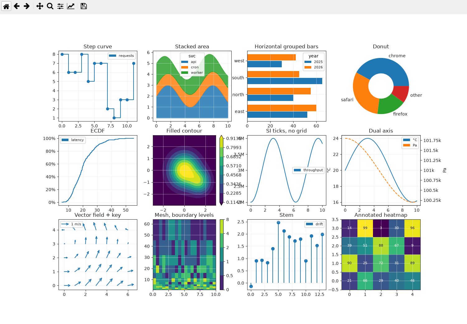
An immutable plot vocabulary, each element pure data:

qv.Scatter(table, x="x", y="y", color_by="category")
qv.Curve(table,   x="t", y="v", step="post", marker="circle")
qv.Curve(table,   x="t", y="v", color_by="regime")            # per-segment coloring
qv.Bars(table,    x="category", y="count", by="region", orient="horizontal",
        annotate="auto")                                    # value labels on bars
qv.Area(table,    x="t", y="load", by="service", mode="stacked")
qv.Histogram(table, value="value", bins="fd")
qv.Ecdf(table, value="latency")
qv.Stem(table, x="day", y="delta", baseline=0.0)              # lollipop series
qv.Heatmap(table, x="x", y="y", z="z", annotate="auto")    # contrast-aware labels
qv.Image(array2d, extent=(0, 0, 10, 10), norm="log")          # also "power",
qv.Mesh(array2d,  x=xe, y=np.geomspace(1, 64, 13),
        norm=qv.Norm("boundary", levels=[0, 1, 2, 4, 8]))     # one norm spec
qv.Contour(field2d, extent=(0, 0, 10, 10), levels=8, annotate=True)
qv.Quiver(table, x="x", y="y", u="u", v="v", key=10, key_label="10 m/s")
qv.Streamlines({"u": u2d, "v": v2d}, u="u", v="v", extent=(0, 0, 10, 10), density=1.5)
qv.Pie(table, value="share", by="browser", hole=0.4)
qv.ErrorBars(table, x="x", y="y", err="sigma",
             lo_limit="is_lo", hi_limit="is_hi")              # "beyond" arrow caps
qv.Spread(table, x="t", lo="lo", hi="hi")   # filled confidence band
qv.BoxPlot(table, value="score", by="cohort")
qv.Violin(table,  value="score", by="cohort")

Annotations & references share the same tree — lines, spans, shapes, text, arrows, and slope references:

qv.HLine(4.5, label="alarm") ; qv.VLine(0.0) ; qv.Span(2, 4)
qv.Text(5, 2, "peak", rotation=30, frame=True)
qv.Arrow(1, 0.2, 4, 0.8) ; qv.Rect(2, -0.5, 4, 0.5)
qv.Ellipse(5, 0, 1.5, 0.4, angle=20) ; qv.Polygon([(6, 0), (7, 0.6), (8, -0.2)])
qv.RefLine(0.1, -0.2, label="1:10 slope")

Axes

Per-axis AxisSpec on the shared surface; events stay in data space (R1):

qv.Overlay([a, b], options=qv.OverlayOptions(
    title="Spectrum",
    x=qv.AxisSpec(scale="log", lim=(1, 1e4)),
    y=qv.AxisSpec(tick_format="eng"),        # SI ticks; also ".0%", ",d", "%H:%M",
                                             # and templates: "{:.0f} ms", "${:,.0f}"
    y2=qv.AxisSpec(label="Pa"),              # twin right axis — put a series on it
    grid=False,                              # with Curve(..., axis="y2")
))

qv.AxisSpec(ticks=[0, 5, 10], tick_labels=["lo", "mid", "hi"],  # pinned positions
            minor=True, tick_rotation=45)                       # minor ticks, tilt

qv.Curve({"t": dt64_stamps, "v": values}, x="t", y="v")   # datetime64 → calendar
                                                          # ticks on every backend

Composition

Build a figure tree with two operators:

scatter * curve                 # Overlay: same axes, layered
scatter + histogram             # Layout: side-by-side panels
qv.Layout([a, b, c], kind="tabs")                                  # grid | splitter | tabs | dock
qv.Layout([a, b], options=qv.LayoutOptions(cols=2, link_x=True))   # shared X axis
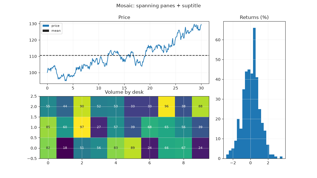
qv.Layout.mosaic("AAB\nCCB", A=a, B=b, C=c)                        # spanning panes from an ASCII plan

Mosaic grids take LayoutOptions(width_ratios=…, height_ratios=…) for track sizes and title= for a figure-level suptitle:

Views & backends

A View is a QWidget; choose an engine or let qtviz pick:

view = qv.View(scatter * curve, backend="auto")   # "pyqtgraph" | "matplotlib" | "webengine"
view.set_backend("matplotlib")                     # swap at runtime — keeps zoom + subscriptions

Typed events

view.on(qv.SelectEvent, lambda e: print(e.indices, e.bounds))   # brush → row indices
view.on(qv.SelectEvent, on_brush, source=scatter)  # scoped to one element
view.on(qv.PickEvent,   lambda e: print(e.point_index, e.x, e.y))
view.on(qv.HoverEvent,  lambda e: print(e.x, e.y, e.value))     # value set on datashaded rasters

Data binding

A channel binds to a column name, a lazy Expression, a callable, or a literal array:

qv.Scatter(df, x="time", y="temp")                          # a column name
qv.Curve(df,   x="time", y=qv.col("raw") - qv.col("base"))  # an Expression (derived, lazy)
qv.Curve(df,   x="time", y=lambda d: d["raw"].cumsum())     # a callable
qv.Scatter({}, x=np.linspace(0, 1, n), y=values)            # literal arrays

Big data — Datashader

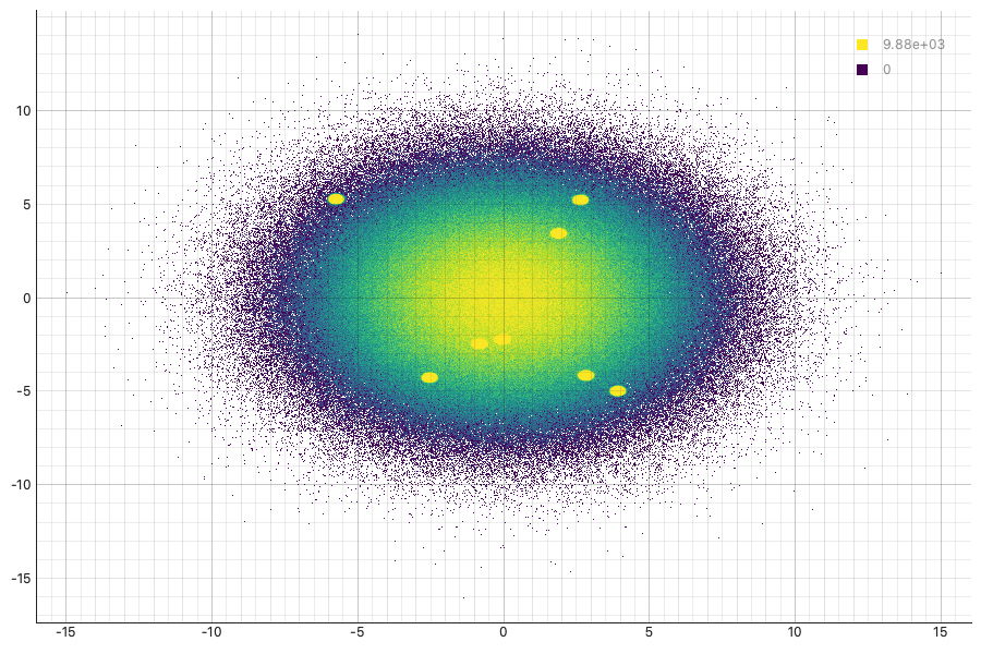
qv.Scatter(big, x="x", y="y", raster="datashader")   # density raster, re-aggregates on zoom
qv.Scatter(big, x="x", y="y", raster="auto")         # rasterize past a threshold
view.on(qv.HoverEvent, lambda e: print(e.value))    # count/mean under the cursor

Reactive

sel = qv.signal([])
filtered = qv.derived(lambda: subset(table, sel.get()))
view = qv.View(filtered)            # re-renders whenever `sel` changes
src.on(qv.SelectEvent, lambda e: sel.set(e.indices))

HoloViews / hvplot

qv.from_holoviews(hv.Scatter(df, "x", "y") * hv.Curve(df, "x", "y"))   # native translation
qv.from_hvplot(df, "scatter", x="x", y="y")                            # pandas .hvplot one-liner

See the Gallery for runnable end-to-end scripts.